About Our Model
About Us
This website was created for the predictions for the upcoming Congressional Elections made by the Political Statistics class at Montgomery Blair High School in Silver Spring, Maryland. Under the guidance of Mr. David Stein, this model (which we named the Overall Results of an Analytical Consideration of the Looming Elections a.k.a. ORACLE of Blair) was developed by a group of around 70 high school seniors, working diligently since the start of September. Apart from the youth and enthusiasm that went into making it, the advantage our model has over professionally developed models is transparency. Unlike professionals, we need not have any secrets in regards to how our predictions are generated. In fact, the sections that follow attempt to detail exactly how we come up with all of the numbers involved in our model. If you are interested by politics, statistics, education, or just agree with our predictions, please tell your friends and social media followers about the work that we’ve done.
Our Methodology
Preliminaries
First, some conventions used throughout the explanation of our methodology. All calculations made are based on the two party vote, meaning that any votes for a third-party or independent candidate do not count. For example, in Oregon's 3rd Congressional District, we say that in 2014 the Democratic vote percentage was \(78.7\%\), even though the Democratic candidate only got \(72.3\%\) of the actual vote. The \(78.7\%\) represents the ratio of votes cast for the Democrat to the total votes cast for either the Republican or the Democrat, hence it’s a two-party vote percentage. The two-party vote percentage differs from the actual vote percentage as some votes are not counted due to the votes being cast for a third-party or an independent candidate.
Another convention used is that, when using a metric centered at \(0\), positive numbers mean a Democratic advantage and negative numbers mean a Republican advantage. For example, when talking about margin in the elections, we usually look at the Democratic margin, as opposed to the Republican Margin. A margin of \(10\%\) means that the Democratic candidate received \(10\%\) more of the two-party vote than the Republican candidate. This means that the Democrat got \(55\%\) of the two-party vote. Going in the other direction, a Democratic margin of \(-20\%\) means that the Democratic candidate received \(20\%\) less of the two-party vote than the Republican Candidate. This means that the Republican candidate prevailed with \(60\%\) of the two-party vote.
BPI and SEER
The Blair Partisan Index (BPI) is a metric that measures a district’s partisan voting tendencies relative to the nation. In order to calculate this, we subtract the national Democratic vote percentage from a district’s Democratic vote percentage for four recent elections: the 2012 and 2016 Presidential elections and the 2014 and 2016 House elections. The subtraction leads to the relative Democratic vote percentages of a district. For example, in AR-02 during the 2016 House election, the district cast \(39\%\) of their two-party vote for the Democratic nominee. In comparison, the nation as a whole cast \(50.57\%\) of their two-party vote for a Democratic nominee.
To be consistent with our predicted 2018 incumbency advantage (weights for SEER), we adjusted 2014 and 2016 House vote proportions based on incumbency in those years. Specifically, if there was a Democratic incumbent running we subtracted \(3.45\%\) (\(6.90\%/2\)) from the Democratic vote proportion and if there was a Republican incumbent running we added \(4.09\%\) (\(8.17\%/2\)) to the Democratic two-party vote proportion. So in 2016, there was a Republican incumbent running for the House for AR-02. Therefore, we added \(4.09\%\) to the district's Democratic vote percentage leading to an adjusted vote percentage of \(39\% + 4.09\% = 43.09\%\) for the 2016 House election. We then take the adjusted vote percentage and subtract it from the national average of \(50.57\%\) to get a relative 2016 House vote percentage of \(43.09\% - 50.57\% = -7.48\%\). The BPI is a weighted average of the relative vote percentages, weighted by the table below:
|
Relative 2012 Presidential Vote Weight: |
0.133 |
|
Relative 2014 House Vote Weight: |
0.278 |
|
Relative 2016 Presidential Weight: |
0.244 |
|
Relative 2016 House Weight: |
0.345 |
The BPI of a district with relative vote percentages \( v_1, v_2, v_3, v_4 \) is \( 0.133v_{1}+0.278v_{2}+0.244v_{3}+0.345v_{4} \). So for AR-02, the BPI would be \(0.133(-8.01\%) + 0.278(-1.35\%) + 0.244(-6.79\%)+0.345(-7.48\%)\), which is \(-5.68\%\).
Districts in which the 2014 and/or 2016 House elections did not have both a Democratic candidate and a Republican candidate pose a problem, since only one major party has a vote total, and that vote total is not meaningful. Therefore, if a past race was unopposed we did not use it in calculating that district's BPI. That is to say, we calculated the BPI as the weighted average of only the races with candidates from both major parties, using the above weights for each election and dividing the weighted sum by the sum of the weight for the elections used. As an example, consider AR-04, where there was no Democratic candidate for the House seat in 2016. AR-04 has relative vote percentages of \(-15.22\%\) for Obama in 2012, \(-2.85\%\) for the Democratic House candidate in 2014, and \(-18.33\%\) for Clinton in 2016. There was no incumbent running for the House seat in 2014, so no adjustment is needed. The BPI of AR-04 is therefore \(0.133(-15.22\%)+0.278(-2.85\%)+0.244(-18.33\%)/(0.133+0.278+0.244)=-14.39%\)
The Synthesized using Earlier Elections as Rationale (SEER) percentage is the first forecast given by the ORACLE of Blair process. SEER begins with a prediction of the Democratic margin, or by how much of the two-party vote the Democratic nominee will win or lose. The Democratic margin prediction is a scale of the BPI shifted by incumbency, incumbency being whether or not a Democratic or a Republican incumbent is running. The scale of the BPI and the shift based on incumbency are listed below:
|
Partisanship Weight: |
2 |
|
Dem Incumbency Weight: |
6.90% |
|
Rep Incumbency Weight: |
8.17% |
By our positive-negative convention, we subtract \(8.17\%\) if a Republican incumbent is running and add \(6.90\%\) if a Democratic incumbent is running. So, as AR-02 has a BPI of \(-5.68\%\) and a Republican incumbent running, SEER predicts a Democratic margin of \(2 (-5.68\%) - 8.17\% = -19.63\%\), meaning SEER predicts that the Democratic nominee will lose by \(19.63\%\) of the two-party vote. This leads to the final SEER prediction of the Democratic two-party vote, which is calculated by \(50\% + 0.5 (margin)\). So for AR-02 SEER predicts that \(50\% + 0.5(-19.63\%) = 40.24\%\) of the two-party vote will go to the Democratic nominee.
We also assigned a standard deviation to each SEER prediction. Based on some tests of the predictive accuracy of past election results, we used a standard deviation of \(0.066\) if there is an incumbent (of either party) running in 2018 and \(0.074\) if there is not. These standard deviations are for the two-party vote proportion predictions.
National Mood Shift (bigmood)
To calculate and adjustment for the national mood, we started with an estimation of the expected major-party voter turnout in 2018. To get this, we started with the sum of Democratic and Republican voters in each Congressional election in 2014. In cases where the 2014 turnout in a district was problematic due to their not being a contested House race (leading to low vote totals) or due to redistricting, we used the 2016 turnout in that district scaled down by the ratio of 2014 average contested district turnout to 2016 average contested district turnout (which is less than 1). In cases where the 2016 turnout is also problematic, we resorted to using the average 2014 turnout for those districts. We then determined, based on our SEER predictions for each district and the number of expected major-party voters in each district, the predicted total number of Democratic and Republican votes on the national level, from which we get the predicted national two-party Democratic vote.
We then compare this to current generic ballot polls. Generic ballot polls ask respondents nationwide whether they plan to vote for the Democratic Congressional candidate or for the Republican Congressional candidate in their districts without naming the candidate. We use a weighted average of generic ballot polls, averaged using the same method as used for polls in an individual district (discussed below); the weighted average Democratic two-party vote is referred to here as the current National Mood. We then find the difference between the current National Mood and the National fundamental prediction discussed in the first paragraph. Let us call this difference the National Mood Shift.
Each district has an elasticity (taken from 538), which quantifies how much more or less than the national average a district is affected by shifts in the national mood. The average elasticity is \(1.00\) (affected the same as the country as a whole). For example, the Democratic vote percentage of a hypothetical district with elasticity \(0.90\) is expected to shift by \(0.9\) points for every 1-point shift in the National Mood, in the same direction as the national mood.
To combine the National Mood with the SEER predictions, we add the product of the National Mood Shift and the elasticity for each district to the SEER prediction for the district to get the bigmood prediction for each district.
There are two sources of variation of the shift. The first the generic ballot polling average. The standard deviation of the polling average (\(\sigma_{p}\)) isn’t calculated from the standard deviation of the individual polls, but rather from looking at the relationship between generic ballot average and national popular House vote from 2002 to 2016. This yields a (\(\sigma_{p}\)) of \(1.38\) percentage points. The second source of variation is the variation of the SEER predictions, which persists when they are applied to the 2014 voter turnout. The standard deviation (\(\sigma_{q}\)) of the SEER-based projected national vote is therefore:
$$\sigma_{q} = \frac{\sqrt{\sum\limits_{i=1}^{435} t_{i}^{2}+\sigma_{i}^{2}}}{\sum \limits_{i=1}^{435} t_{i}}$$
Where the \(i\)th district (from \(1\) to \(435\)) has 2014 two-party turnout \(t_{i}\) and the SEER standard deviation for the ith district has standard deviation \(\sigma_{i}\). The overall standard deviation of the national mood shift is given by \(\sqrt{\sigma_{p}^{2}+\sigma_{q}^{2}}\).
Averaging polls
For districts that have polls for their congressional races, we construct a weighted average of those polls. We start by getting for each poll: the two-party Democratic vote prediction \((0 < p < 1)\), the number of days before the election that the poll was finished (\(t\)), and the sample size of the poll (\(n\)). The polls are weighted by their ages, based on the relative values of this function for the different ages of the polls:
$$f(t)=e^{-t/30}$$
Therefore, if there are \(m\) polls in a district, and the \(a\)th poll is from \(t_{a}\) days before the election, it will have weight \(w_{a}\):
$$w_{a}=\frac{e^{\frac{-t_{a}}{30}}}{\sum\limits_{i=1}^m e^{\frac{-t_{i}}{30}}}$$
This ensures that old polls are weighted less than newer polls, that the marginal penalty for being one day older decreases as the polls get older, and that the weights sum to \(1\). We then get the weighted average of the predictions by summing the products of each poll’s predicted Democratic two-party vote proportion and that poll’s weight. However, there is some variation in polls which we include as uncertainty in our model. One source of this variation is sampling error. Given a poll with Democratic vote share \(p\), Republican vote share \((1-p)=q\), and sample size \(n\), the average sampling error \(se\) of such a poll is given by:
$$se=\sqrt{\frac{pq}{n}}$$
For now, we will say that the standard deviation \(\sigma\) of each poll (i.e. the average error) is its sampling error.
However, there are other sources of variation that we are unable to empirically calculate. We divide the polls into four grades (A, B, C, and D; taken from 538) based on the quality of the pollster’s methodology. For each grade of polls, we took polls from previous House elections (starting in 2012) and found the average distance around the line of best fit for actual election results vs. poll results (i.e. the line that best predicted the actual election result given a poll result). Let’s call this average distance the past poll standard deviation for each grade.
We then find the average sampling error of all polls of each grade. For each grade, we then add ((past poll standard deviation) - (average sampling error)) to the standard deviation of each poll with that grade. Although the numbers will change slightly as we add more polls with slightly different average sampling errors, we found that the average sampling error is generally between \(0.02\) and \(0.025\) regardless of grade. Here are approximate standard deviation increases for each grade:
|
Grade |
Standard Deviation Around Regression Line |
Est. Standard Deviation Increase |
|
A |
0.0565 |
0.034 |
|
B |
0.0662 |
0.044 |
|
C |
0.0767 |
0.054 |
|
D |
0.1303 |
0.105 |
Given two polls \(P_{1}\) and \(P_{2}\) with standard deviations \(\sigma_{2}\) and weights \(w_{1}\) and \(w_{2}\), we can find the standard deviation of the weighted sum of \(P_{1}\) and \(P_{2}\) with:
$$\sigma_{1}+\sigma_{2}=\sqrt{w_{1}^{2}\sigma_{1}^{2}+w_{2}^{2}\sigma_{2}^{2}}$$
This can be generalized to more than two polls to get one ‘weighted average’ standard deviation for the weighted average of the polls in a district.
Weighting Polls vs Bigmood
For districts with polls, we take a weighted average of the bigmood prediction and aggregate poll prediction to get to our final prediction. The weight (\(0 < weight < 1\)) of the polls depends on 1) the number of polls, 2) the grade of each poll, and 3) the age (in days before the election) of each poll. We first calculate the Grade Point Sum (GPS) of all of the polls. If a district has \(m\) polls, and the \(i\)th poll has grade \(g_{i}\) and is from \(t_{i}\) days before the election, the GPS is:
$$GPS=\sum\limits_{i=1}^m G(g_{i})e^{\frac{-t_{i}}{167}}$$
Where \(G(g_{i})\) is \(0.177\) if \(g_{i}\) is A, \(0.151\) if \(g_{i}\) is B, \(0.130\) if \(g_{i}\) is C, and \(0.077\) if \(g_{i}\) is D.
The weighting of the aggregate poll prediction (\(w_{p}\)) is then given by:
$$w_{p}=\frac{1.9}{\pi} \cdot \arctan(6.12 \cdot GPS)$$
And the weighting of the bigmood prediction is (\(1-w_{p}\)).
The constants of the arctan function were chosen so that it has an asymptote of \(0.95\) (a district with a very large GPS has a poll weight very close to \( 0.95\)) and so that a district with two B polls, each finished the day of the election, will have poll weight \(0.6\).
Blairvoyance
Blairvoyance provides a hypothesized poll result for districts without polls by interpolating on demographics of the districts that do have polls. First, Blairvoyance creates linear relationships between districts using select demographics for that district. Figure 1 is a simplified example where the three districts are plotted against two axes representing two demographics, which is effectively a representation of a relationship between districts.
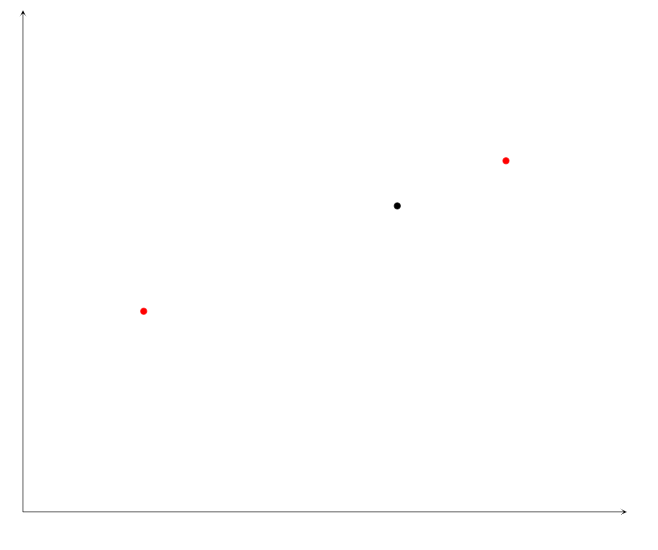
Figure 1. Blairvoyance demographics mapping
The closer they are in Figure 1, the more similar the districts by some metric formed by the demographic data. The red dots represent the districts with polling data. Blairvoyance then moves the points that represent district with polls to another dimension, which represent the poll result. Figure 2 is a representation of Figure 1 with the third axes of poll result is added, and Figure 3 shows the points being moved into the third dimension representing polls.
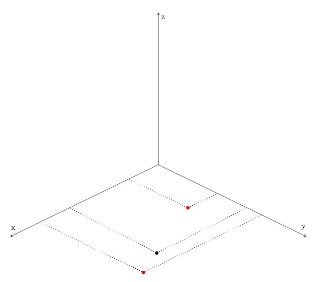
Figure 2. Blairvoyance mapping in 3-space
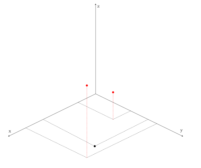
Figure 3. Blairvoyance adding in poll results
Keep in mind that, our model contains more than two demographics, therefore Blairvoyance utilizes more than 3-dimensions. Blairvoyance then tries to fit a curve relating demographics and poll results. The blue line in Figure 4 represents a potential fitted curve Blairvoyance might create in that simplified case. Then, in order to create a hypothesized poll result for a district without poll, it will use the poll result of the closest poll in the fitted curve, as can be seen in Figure 5.
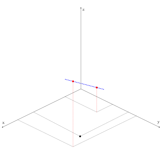
Figure 4. Blairvoyance curve fitting
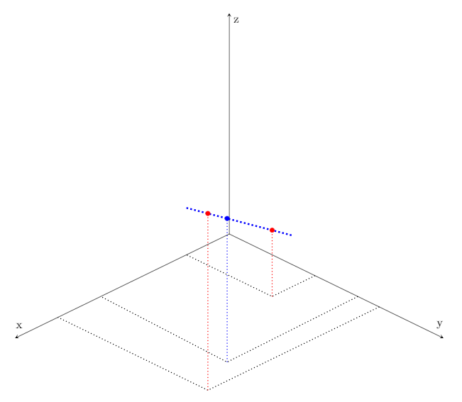
Figure 5. Blairvoyance poll hypothesis
Blairvoyance takes in polls and returns poll hypotheses. Typically, polls are only done on the districts with close races. Therefore, Blairvoyance should make poll hypotheses closer than actual polls would be; the weight of Blairvoyance should decrease as partisanship increases. Hence, the weight of Blairvoyance should be at most the best poll we can have, which is an A graded poll taken one day before the election. Let the weight of one A graded poll taken one day before election be \(w_a\). Then the weight of Blairvoyance would be \(w_a (1 + 2|bigmood - 0.5|)\). This satisfies both properties that it is at most \(w_{a}\) and decreases as partisanship increases. If some hypothetical district is completely partisan, Blairvoyance would not count toward the prediction of that district.
Calculating AUSPICE
The Agglomeration Utilizing Statistical Predictions and Inquiries Concerning Elections (AUSPICE) is the final election forecast that the ORACLE of Blair gives a district every run. AUSPICE is a combination of the distribution provided by Bigmood and the averaged polls, or Blairvoyance in the absence of polls, weighted as mentioned above. Suppose the weight of bigmood is \(w_b\) and the weight of the averaged polls for a district (or Blairvoyance) to be \(w_l\). And suppose that bigmood gives a mean of \(\mu_b\) and a standard deviation of \(\sigma_b\) for the proportion of the two-party vote going to the Democratic nominee, and the polls give a mean of \(\mu_l\) and a standard deviation of \(\sigma_l\). The AUSPICE for that district will return a mean of \(w_l \mu_l + w_b \mu_b\) and a standard deviation of \(\sqrt{(w_l \sigma_l)^2+(w_b \sigma_b)^2}\).
National Predictions
At this point, we have predicted vote shares and standard deviations of vote shares, so it might seem that calculating the overall chance that a party gets a majority of seats is rather simple. However, this is not the case.
In order to avoid excessive computations or calculating an exact number, we simulate the entire House election \(10,000,000\) times each time we run our model. The probability that each party wins a majority of seats in the House is then about the number of simulations in which this happens divided by \(10,000,000\).
A naïve approach to use here would be to simulate each district separately, using the numbers we already have. However, this approach has the implicit assumption that the district vote shares are all independent, which is certainly not the case. For one, the systematic bias of polls can often be caused by the same factors from district to district. Also, since our model is not perfect, it may be consistently off in one direction for most districts. Thus, our simulation must introduce some correlation between districts.
The way we chose to implement this is to, for each simulation, choose a number \(s\) from a normal distribution with mean \(0\) and variance \(\sigma^2\) (we will explain where \(\sigma\) comes from later). Then, for every district \(d\) with mean vote share \(\mu_d\) and variance of the vote share \(\sigma_d^2\), we choose a number \(v_d\) from a normal distribution with mean vote share \(\mu_d\) and variance \(\sigma_d^2 - \sigma^2\) and let the simulated vote share be \(v_d + s\). Since \(v_d\) and \(s\) are independent, this means that the distribution of \(v_d + s\) has mean \(\mu_d\) and variance \(\sigma_d^2\), matching our earlier computations The important part is that \(s\) is the same for all districts, meaning that a portion of the variance of the districts is shared.
It suffices to find a suitable value for \(\sigma\). There is no clear way to do this, but we decided on the following: the outcome of the House is very correlated with the House popular vote, so a good choice for \(\sigma\) is one such that the resulting distribution of the House popular vote matches our uncertainty about it. Since the individual district variation (on the order of \(\sigma \sim 5\%\)) is all independent, the contribution to the House popular vote from these sources of variation is on the order of \(5\%/\sqrt{435} \sim 0.25\%\) which is far lower than the actual uncertainty. So we should have \(\sigma\) be our uncertainty about the House popular vote.
There are many ways to forecast the House popular vote, but using the standard deviation of the national voter turnout prediction is close to the best one can do. Therefore, we use the historical standard deviation of the national generic ballot polls versus the national popular vote, which corresponds to \(\sigma \approx 1.38\%\).
Example: California’s 25th District
Please note that in this example calculations may be shown with intermediate rounding. However, the actual computations used to produce results did not use intermediate rounding. This district is currently represented by Republican Steve Knight. He is being challenged by Democrat Katie Hill. This section was updated on October 26th.
BPI
Obama received \(49.1\%\) of the two-party vote in this district in 2012. As a consequence of California’s jungle primary system, there was no Democrat on the 2014 House ballot. We therefore used the aggregate two-party Democratic performance in the jungle primary, which was \(32.8\%\); there was no incumbent running in 2014. Clinton received \(53.6\%\) of the two-party vote in this district in 2016. There was a Democratic candidate for the House seat in 2016 and he got \(46.9\%\) of the vote; there was a Republican incumbent. Since there was a Republican incumbent in 2016, we adjust the Democrat’s vote share in 2016 to be \(51.0\%\).
This district thus has a BPI of \(0.133(49.1-50) + 0.278(32.8-50) + 0.244(53.6-50)+0.345(51.0-50) = -3.59\%\). Therefore, as there is a Republican incumbent running in 2018, this district has a SEER prediction of \(50\% + 0.5(2(-3.59\%) - 8.17\%) = 42.4\%\). Since there is an incumbent, we will use a standard deviation of \(0.066\) for the SEER prediction.
Bigmood
Using the SEER predictions and procedure described above in the National Mood Shift section, our nationwide fundamental prediction with a 2014 turnout model is that Democrats would get \(49.5\%\) of the two-party vote. The current (at the time or writing) generic ballot average is that Democrats will get \(54.3\%\) of the two-party vote. This implies an average shift of \(+4.8\%\) to the Democratic two-party votes in each district to get the big mood predictions. This number will change as more generic ballot polls are conducted, but it is suitable for this example. CA-25 has an elasticity of \(0.97\), so it has a bigmood prediction of \(42.4\% + 0.97 \cdot 4.8\% = 47.1\%\).
Polling
This district has six polls:
|
Poll # |
Grade |
Age (days) |
Poll result |
Sample size |
|
1 |
D |
44 |
0.521 |
650 |
|
2 |
A |
48 |
0.489 |
500 |
|
3 |
C |
117 |
0.500 |
400 |
|
4 |
C |
138 |
0.421 |
400 |
|
5 |
B |
264 |
0.556 |
283 |
|
6 |
B |
282 |
0.570 |
650 |
The standard deviation and weight of each poll are:
|
Poll # |
Standard Deviation |
Poll weight function |
Poll weight |
|
1 |
0.125 |
0.231 |
0.498 |
|
2 |
0.056 |
0.202 |
0.436 |
|
3 |
0.079 |
0.020 |
0.044 |
|
4 |
0.079 |
0.010 |
0.022 |
|
5 |
0.074 |
0.000 |
0.000 |
|
6 |
0.063 |
0.000 |
0.000 |
These variances include the sampling error and the grade-based standard deviation increase discussed above in the Averaging Polls section. The weighted average of the polls is approximately \(0.498 \cdot 0.521+0.436 \cdot 0.489+0.044 \cdot 0.500+0.022 \cdot 0.421+0.00 \cdot 0.556+0.00 \cdot 0.570 = 0.504 = 50.4\%\). The weighted average has a standard deviation of approximately \(\sqrt{0.498^{2} \cdot 0.125^{2} + 0.436^{2} \cdot 0.056^{2} + 0.044^{2} \cdot 0.079^{2} + 0.022^{2} \cdot 0.079^{2} \cdot 0.000^{2} \cdot 0.074^{2} + 0.000^{2} \cdot 0.063^{2}} = 0.067\).
Poll Weighting
This district’s polls have \(GPS = 0.077e^{\frac{-44}{167}}+0.177e^{\frac{-48}{167}}+0.130e^{\frac{-117}{167}}+0.130e^{\frac{-138}{167}}+0.151e^{\frac{-264}{167}}+0.151e^{\frac{-282}{167}} = 0.372\). Therefore, the polls in this district have weight \(\frac{1.9}{π} \cdot \arctan(6.12 \cdot 0.372) = 0.70\). The bigmood prediction consequently has weight \(1-0.70 = 0.30\).
Final Prediction
The final prediction for CA-25 is that Hill will get on average \(0.70 \cdot 50.4\% + 0.30 \cdot 47.1\% = 49.4\%\) of the two-party vote. This has a standard deviation of \(\sqrt{0.70^{2} \cdot 0.067^{2} + 0.30^{2} \cdot 0.066^{2}} = 0.051\). Therefore, Hill getting at least \(50\%\) of the two-party vote has a \(z\)-score of \(z = \frac{0.50-0.494}{0.051} = 0.11\). This implies a win probability of \(45.4\%\). In other words, if this particular general election were held a very large number of times, we would expect Hill to win \(45.4\%\) of the time and Knight to win \(54.6\%\) of the time.