Almost all of the Blair ORACLE model is based on publicly available data and transparent formulas which are included on our methodology page. However, our weighting of how much the national mood should shift a given district is based on publicly available “elasticity” scores from FiveThirtyEight. Some of us were concerned with this inclusion as we did not have a complete understanding of the score’s derivation.
We decided to evaluate the accuracy of our implementation of FiveThirtyEight’s elasticity scores by applying them to historical elections.
Our model currently uses elasticity as follows: we calculate each district’s BPI based on the past two House elections and the past two Presidential elections. From this value we calculate an expected Democrat vote percent for each district. Using a 2014 turnout model, we calculate the expected number of Democrat voters in each district. We sum the votes over all districts and divide the sum by the total voting population to determine our fundamental popular vote prediction. We use polls of the generic ballot to estimate the actual popular vote, then we know we must adjust our fundamental predictions for each district to create the correct popular vote.
$$SHIFT = GENERIC - FUNDAMENTAL\_TOTAL$$
A naive approach would be to uniformly shift each district by the difference between the fundamentals predicted popular vote and the poll predicted popular vote. This ignores the issue that certain districts have a greater propensity to shift from their baseline vote than others; some districts are more “elastic”. To resolve this issue, our model multiplies the overall shift by a district’s elasticity as determined by 538 to determine that district’s shift.
$$SHIFT\_ADJ = ELASTICITY * SHIFT$$
However, we noticed after the implementation of the model that this approach is fundamentally flawed. FiveThirtyEight standardizes its elasticity scores to have a national average of exactly 1. Our implementation of elasticity does NOT require this. For example, consider a hypothetical country with just two districts: district A has voting population 100, and district B has voting population 10. Say we find that the national shift should be 10%. We want 11 more votes overall. Say district A has elasticity 0.9, meaning \(0.9*10\%*100 = 9\) additional votes will come from district A. We then know the other two additional votes must come from district B, so \(elasticity*10\%*10 = 2\). This means that district B has elasticity 2. 0.9 and 2 do NOT average to 1, despite being the correct elasticity scores for this election. This is obviously an extreme example, but it illustrates the fact that setting average elasticity to 1 ignores the differences in voting population between districts.
We determined historically correct elasticity for past years using with the same calculations as we are using for the current year. For each year, we first calculated BPI using the two House and Presidential elections prior to that year. We then calculated the expected Democrat vote percent for each district and, using the same 2014 turnout model, calculated the fundamental popular vote. Solving for elasticity, we get that for each year it should equal the difference between actual House Democrat percent for that year and the fundamental Democrat percent, divided by the difference between the popular vote for that year minus the popular vote predicted by fundamentals alone.
$$ELASTICITY = (HOUSE\_RESULT - DISTRICT\_FUND) / (POP\_VOTE - FUND\_TOTAL)$$
Let’s use 2014’s race in Arizona’s 2nd district as an example. The Democratic congressional candidate in this district in 2012 received 50% of the vote. In 2012, Obama received 49% of the vote in this district. In 2010, the Democratic congressional candidate received 32% of the vote. In 2008, Obama received 41% of the vote. We calculate the BPI for this distict using the formula which can be found in our methodology:
$$BPI = 0.345*0.50 + 0.244*0.49 + 0.278*0.32 + 0.133*0.41 = 0.436$$
Using the same formula in our methodology, we convert this BPI into the predicted democratic margin for this district, accounting for incumbency in 2014:
$$DEM\_MARGIN = 0.436*2 + 0*0.0817 + 1*0.0682 = -0.05458480272$$
From there, calculating the democratic vote percentage is simple: \(DEM\_VOTE = -0.05458/2 + 0.5 = 47%\). Now we can calculate what the elasticity should have been in order to adjust the fundamental percentage using the national mood to perfectly predict the House election outcome. Looking back at 2014 data, we find that the democratic candidate actually received 50% of the vote. The House popular vote for 2014 was 47.05%. Using the 2014 turnout model and fundamental percentages, we calculated a predicted House popular vote for 2014 of 49.48%. Plugging these values into the formula for elasticity given above, we get:
$$ELASTICITY = (0.5 - 0.47) / (0.4705 - 0.4948) = -1.12$$
You may find it surprising that elasticity for this district is negative; this implies that this district voted against the national mood. This is fine—we’ll go into more detail about this later.
We wanted to compare our elasticity results with FiveThirtyEight’s values. We found a 1.9% correlation coefficient between our average elasticity from 2006-2016 and FiveThirtyEight’s elasticity, which means that 0.0% of the variation in historical elasticity can be explained by FiveThirtyEight’s.

There is clearly an issue here. The lack of correlation between FiveThirtyEight’s elasticity historical elasticity implies that ORACLE has been heavily shifting districts that don’t actually tend to sway toward the national mood much and barely adjusting districts which tend to sway a lot. In the end, we get an adjusted popular vote that matches the generic ballot for the current year, but to do so we have adjusted the wrong districts in the wrong way. However, it’s possible that elasticity fluctuates greatly between years. In this case, the lack of correlation is less disturbing.
There are a few assumptions and sources of error in our analysis, the biggest of which is redistricting: elasticity calculations between election years are often not comparable if redistricting occurred in the last four years. Another issue is missing data for certain years in certain districts due to our time constraints; we don’t have the resources to manually enter all missing data. In these cases, we chose to average the values of the other years’ data and assume that would be close enough to the missing information. We also assume that elasticity within each district remains relatively constant over time and that the 2014 turnout model is roughly accurate for all years. We will come back to these assumptions in a few paragraphs.
If we only look at our calculations for 2014, many of these issues are mitigated. First, using a 2014 turnout model is necessarily correct for 2014. Second, data is more recent and thus less of it is missing or subject to redistricting. Nonetheless, FiveThirtyEight's elasticity metric has almost no correlation with ours. With a correlation coefficient of r = 12.06, only 1.5% of the variation in 2014 historical elasticity can be explained by FiveThirtyEight’s elasticity.

Let’s look a bit closer at the assumption that elasticity remains fairly constant over time. Below is a box and whisker plot of elasticities for previous years.
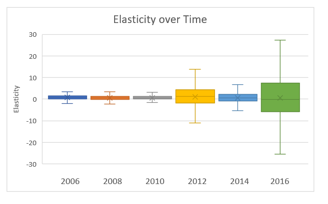
Clearly, the assumption that elasticity remains relatively constant is flawed. Elasticity in Arizona 2 over this time period, for example, was 1.07, 0.75, 0.55, 6.72, -1.12, and then -3.71 — with a standard deviation of 3.437. This implies that elasticity is simply not predictable using historical data, which may explain why FiveThirtyEight did not use historical data to compute their elasticity values. FiveThirtyEight’s elasticity values may be the most accurate values we can use. However, FiveThirtyEight is not transparent about how this value is calculated, which goes against the spirit of our transparent model. We propose removing elasticity from ORACLE and using a uniform shift. We tried running the model with a uniform shift and found that ORACLE’s overall prediction was changed by less than 1%—this is an insignificant difference and would greatly improve the transparency and validity of our model.